Exploratory Data Analysis (EDA) is like being a detective at a party full of numbers. Let’s take the Heart Disease Prediction Dataset as an example.
Imagine you walk into this party, and instead of guests, there are columns of data: ages, blood pressures, cholesterol levels, and so on. Your job as the detective is to mingle with these numbers, get to know them, and uncover their secrets.
You start by looking around to see who’s who. You might notice that the average age of the guests is around 50. Maybe you spot some interesting patterns, like how those with high cholesterol tend to hang out in one corner. You create some cool charts and graphs, which are like taking snapshots of the party. These visuals help you see at a glance who the outliers are—the really tall guy in the middle of a crowd of short folks, or the person who’s overdressed for the occasion.
Occasionally, you overhear intriguing snippets of conversation. For instance, you might hear that smokers are whispering about high blood pressure more than non-smokers. This eavesdropping (or correlation) helps you understand how different variables might be related.
EDA is all about getting a feel for the data without making any big assumptions or trying to prove anything just yet. It’s like being a curious guest at a party, asking questions, spotting trends, and taking notes, all to get a clearer picture of what’s really going on.
Dataset Overview
df = pd.read_csv(Path.cwd() / "heart.csv")
df.info()
<class 'pandas.core.frame.DataFrame'>
RangeIndex: 918 entries, 0 to 917
Data columns (total 12 columns):
 #   Column          Non-Null Count  Dtype
---  ------          --------------  -----
 0   Age             918 non-null    int64
 1   Sex             918 non-null    object
 2   ChestPain       918 non-null    object
 3   RestingBP       918 non-null    int64
 4   Cholesterol     918 non-null    int64
 5   FastingBS       918 non-null    int64
 6   RestingECG      918 non-null    object
 7   MaxHR           918 non-null    int64
 8   ExerciseAngina  918 non-null    object
 9   Oldpeak         918 non-null    float64
 10  ST_Slope        918 non-null    object
 11  HeartDisease    918 non-null    int64
dtypes: float64(1), int64(6), object(5)
memory usage: 86.2+ KB
A brief explanation of each column (taken directly from the Heart Disease Prediction Dataset 😝) is given below:
- Age: age of the patient [years]
- Sex: sex of the patient [M: Male, F: Female]
- ChestPainType: chest pain type [TA: Typical Angina, ATA: Atypical Angina, NAP: Non-Anginal Pain, ASY: Asymptomatic]
- RestingBP: resting blood pressure [mm Hg]
- Cholesterol: serum cholesterol [mm/dl]
- FastingBS: fasting blood sugar [1: if FastingBS > 120 mg/dl, 0: otherwise]
- RestingECG: resting electrocardiogram results [Normal: Normal, ST: having ST-T wave abnormality (T wave inversions and/or ST elevation or depression of > 0.05 mV), LVH: showing probable or definite left ventricular hypertrophy by Estes’ criteria]
- MaxHR: maximum heart rate achieved [Numeric value between 60 and 202]
- ExerciseAngina: exercise-induced angina [Y: Yes, N: No]
- Oldpeak: oldpeak = ST [Numeric value measured in depression]
- ST_Slope: the slope of the peak exercise ST segment [Up: upsloping, Flat: flat, Down: downsloping]
- HeartDisease: output class [1: heart disease, 0: Normal]
As we can see, the dataset contains 918 samples, each characterized by 11 distinct features. The features Sex, ChestPain, FastingBS, RestingECG, ExerciseAngina, and ST_Slope are categorical. We’ll use LabelEncoder to convert these into numerical values. We’ll create a separate encoder for each feature and store them in a dictionary for future use.
target_variable = "HeartDisease"
categorical_features = ["Sex", "ChestPain", "FastingBS", "RestingECG", "ExerciseAngina", "ST_Slope"]
numerical_features = set(df.columns).difference([target_variable, *categorical_features])

encoders = {}
for column in categorical_features:
    encoder = LabelEncoder()
    df[column] = encoder.fit_transform(df[column])
    encoders[column] = encoder
information = df.describe().T
missing = df.isna().sum(axis=0).rename("Missing Values")
unique = df.nunique().rename("Unique Values")

pd.concat([information, missing, unique], axis=1)
| count | mean | std | min | 25% | 50% | 75% | max | Missing Values | Unique Values | |
|---|---|---|---|---|---|---|---|---|---|---|
| Age | 918.0 | 53.510893 | 9.432617 | 28.0 | 47.00 | 54.0 | 60.0 | 77.0 | 0 | 50 |
| Sex | 918.0 | 0.789760 | 0.407701 | 0.0 | 1.00 | 1.0 | 1.0 | 1.0 | 0 | 2 |
| ChestPain | 918.0 | 0.781046 | 0.956519 | 0.0 | 0.00 | 0.0 | 2.0 | 3.0 | 0 | 4 |
| RestingBP | 918.0 | 132.396514 | 18.514154 | 0.0 | 120.00 | 130.0 | 140.0 | 200.0 | 0 | 67 |
| Cholesterol | 918.0 | 198.799564 | 109.384145 | 0.0 | 173.25 | 223.0 | 267.0 | 603.0 | 0 | 222 |
| FastingBS | 918.0 | 0.233115 | 0.423046 | 0.0 | 0.00 | 0.0 | 0.0 | 1.0 | 0 | 2 |
| RestingECG | 918.0 | 0.989107 | 0.631671 | 0.0 | 1.00 | 1.0 | 1.0 | 2.0 | 0 | 3 |
| MaxHR | 918.0 | 136.809368 | 25.460334 | 60.0 | 120.00 | 138.0 | 156.0 | 202.0 | 0 | 119 |
| ExerciseAngina | 918.0 | 0.404139 | 0.490992 | 0.0 | 0.00 | 0.0 | 1.0 | 1.0 | 0 | 2 |
| Oldpeak | 918.0 | 0.887364 | 1.066570 | -2.6 | 0.00 | 0.6 | 1.5 | 6.2 | 0 | 53 |
| ST_Slope | 918.0 | 1.361656 | 0.607056 | 0.0 | 1.00 | 1.0 | 2.0 | 2.0 | 0 | 3 |
| HeartDisease | 918.0 | 0.553377 | 0.497414 | 0.0 | 0.00 | 1.0 | 1.0 | 1.0 | 0 | 2 |
At first impression, we can see that:
- Fortunately, the dataset contains no missing values, so there is no need for imputation or deletion of rows.
- All features exhibit a relatively high standard deviation, suggesting that low variance elimination methods like
VarianceThresholdmay not be suitable. - The value ranges of individual feature distributions vary significantly. We need to examine each feature to determine if it follows a normal distribution and to identify any outliers.
Dataset Balance
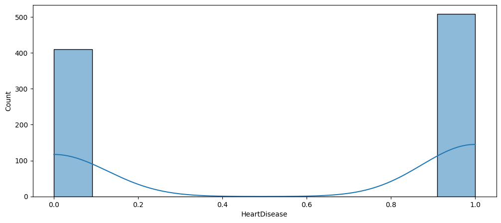
As shown below the dataset is relatively balanced. If that wasn’t the case, we might had to employ an oversampling technique, such as SMOTE.
Feature Distribution & Outliers
To effectively train our model, it’s crucial to analyze the distribution of each feature and identify any outliers. Based on these findings, we can decide whether to use StandardScaler or RobustScaler to normalize the features appropriately. The MinMaxScaler might be worth considering if the features are not Gaussian. However, it is probably not the most suitable option since it assumes features are bounded within a specific range, which is not the case.
We know that categorical variables are inherently non-continuous and thus cannot follow a normal distribution. However, we can assess the distribution of continuous features to determine if they approximate a normal distribution.
Furthermore, the concept of outliers in categorical data is somewhat problematic. To identify an outlier, there needs to be a measure of difference between data. Taking this into consideration, we will exclude categorical features from our outlier detection process.
num_features = len(numerical_features)
num_cols = 2
num_rows = (num_features // num_cols) + int(num_features % num_cols != 0)

fig, axes = plt.subplots(num_rows, num_cols, figsize=(15, 5 * num_rows), constrained_layout=True)

axes = axes.flatten()

for i, feature in enumerate(numerical_features):
    sns.histplot(data=df, x=feature, kde=True, stat="density", ax=axes[i])
    axes[i].set_xlabel(feature)
    axes[i].set_ylabel('Density')

for j in range(i + 1, len(axes)):
    fig.delaxes(axes[j])

plt.show()
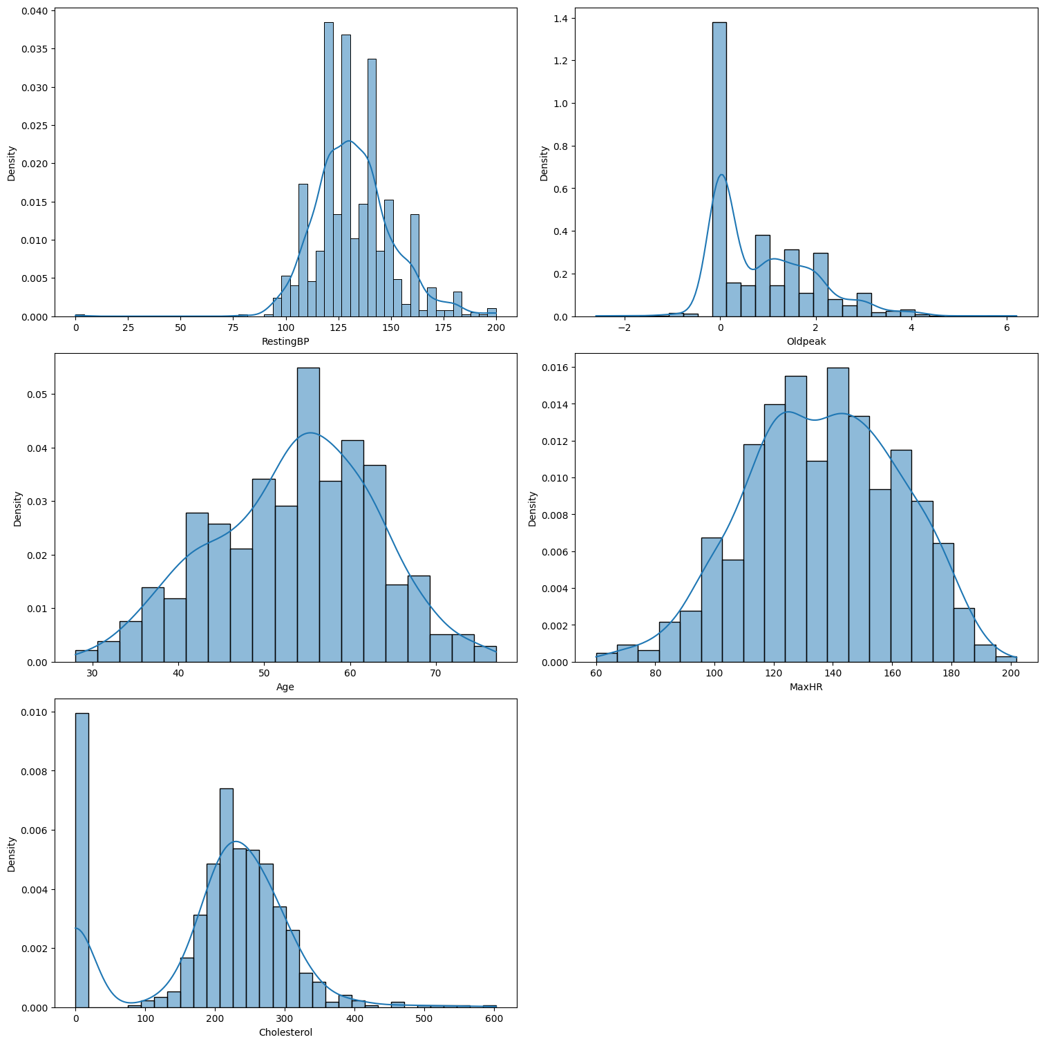
Based on our analysis, we can draw the following conclusions:
- Age and MaxHR appear to follow a normal distribution.
- Oldpeak is right-skewed.
- Cholesterol exhibits a bimodal distribution.
- RestingBP might follow a normal distribution, but its high variability prevents us from determining this with certainty.
It is evident that the StandardScaler is probably not be suitable in this case.
num_features = len(numerical_features)
num_cols = 2
num_rows = (num_features // num_cols) + int(num_features % num_cols != 0)

fig, axes = plt.subplots(num_rows, num_cols, figsize=(15, 5 * num_rows), constrained_layout=True)

axes = axes.flatten()

for i, feature in enumerate(numerical_features):
    sns.boxplot(data=df, y=feature, hue="HeartDisease", ax=axes[i], gap=.1)
    axes[i].set_xlabel(feature)
    axes[i].set_ylabel('Density')

for j in range(i + 1, len(axes)):
    fig.delaxes(axes[j])

plt.show()
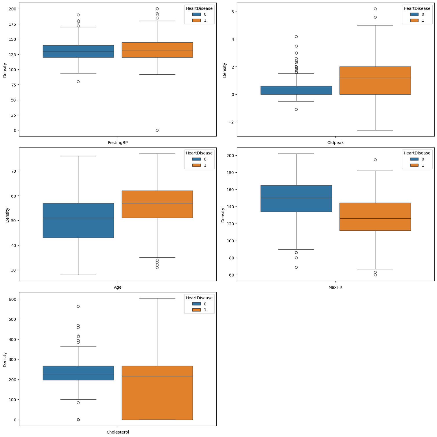
It is evident that all features, exhibit at least some outliers. Consequently, we will apply the RobustScaler for feature normalization to address these outliers effectively.
Correlation Analysis
We now analyze the correlation between different features and our target variable, as well as examine the relationships among the features themselves, to gain deeper insights.
num_features = len(categorical_features)
num_cols = 2
num_rows = (num_features // num_cols) + int(num_features % num_cols != 0)

fig, axes = plt.subplots(num_rows, num_cols, figsize=(15, 5 * num_rows), constrained_layout=True)

axes = axes.flatten()

for i, feature in enumerate(categorical_features):
    sns.countplot(data=df, x=feature, hue="HeartDisease", ax=axes[i])
    axes[i].set_xlabel(feature)
    axes[i].set_ylabel('Density')

for j in range(i + 1, len(axes)):
    fig.delaxes(axes[j])

plt.show()
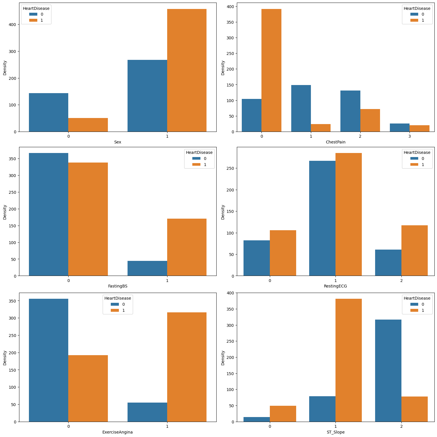
We can see that:
- Male patients are more prone to heart disease compared to female patients.
- Asymptomatic chest pain
ASY (0)is highly indicative of heart disease, while typical anginaTA (3)seems to have minimal effect on outcomes. In contrast, atypical anginaATA (1)and non-anginal painNAP (2)seem to be negatively correlated with heart disease. - A fasting blood sugar greater than 120 mg/dl
(FastingBS = 1)is linked to a higher likelihood of heart disease. On the other hand, a fasting blood sugar less than 120 mg/dl(FastingBS = 0)is only marginally associated with a lower likelihood of heart disease. RestingECGdoes not appear to influence the likelihood of heart disease.- Exercise-induced angina
(ExerciseAngina = 1)is strongly associated with heart disease, while its absence is strongly correlated with a lower likelihood of the condition. - A downward
ST_Slopeshows a slight correlation with heart disease, a flatST_Slopeis strongly correlated, and an upwardST_Slopeis associated with a lower likelihood of heart disease.
RestingECGcould be considered insignificant and will most probably be dropped from the dataset.
We also observe that for some categorical features, certain values are predictive of heart disease, while others show no correlation with the condition (as in the case of FastingBS). To address this, we could apply OneHotEncoder. This technique converts categorical values into binary features, enabling the model to better interpret the presence or absence of specific categories and potentially enhancing predictive accuracy. Additionally, one-hot encoding prevents the algorithm from mistakenly assuming an ordinal relationship among the categories.
num_features = len(numerical_features)
num_cols = 2
num_rows = (num_features // num_cols) + int(num_features % num_cols != 0)

fig, axes = plt.subplots(num_rows, num_cols, figsize=(15, 5 * num_rows), constrained_layout=True)

axes = axes.flatten()

for i, feature in enumerate(numerical_features):
    sns.histplot(data=df, x=feature, hue="HeartDisease", ax=axes[i])
    axes[i].set_xlabel(feature)
    axes[i].set_ylabel('Density')

for j in range(i + 1, len(axes)):
    fig.delaxes(axes[j])

plt.show()
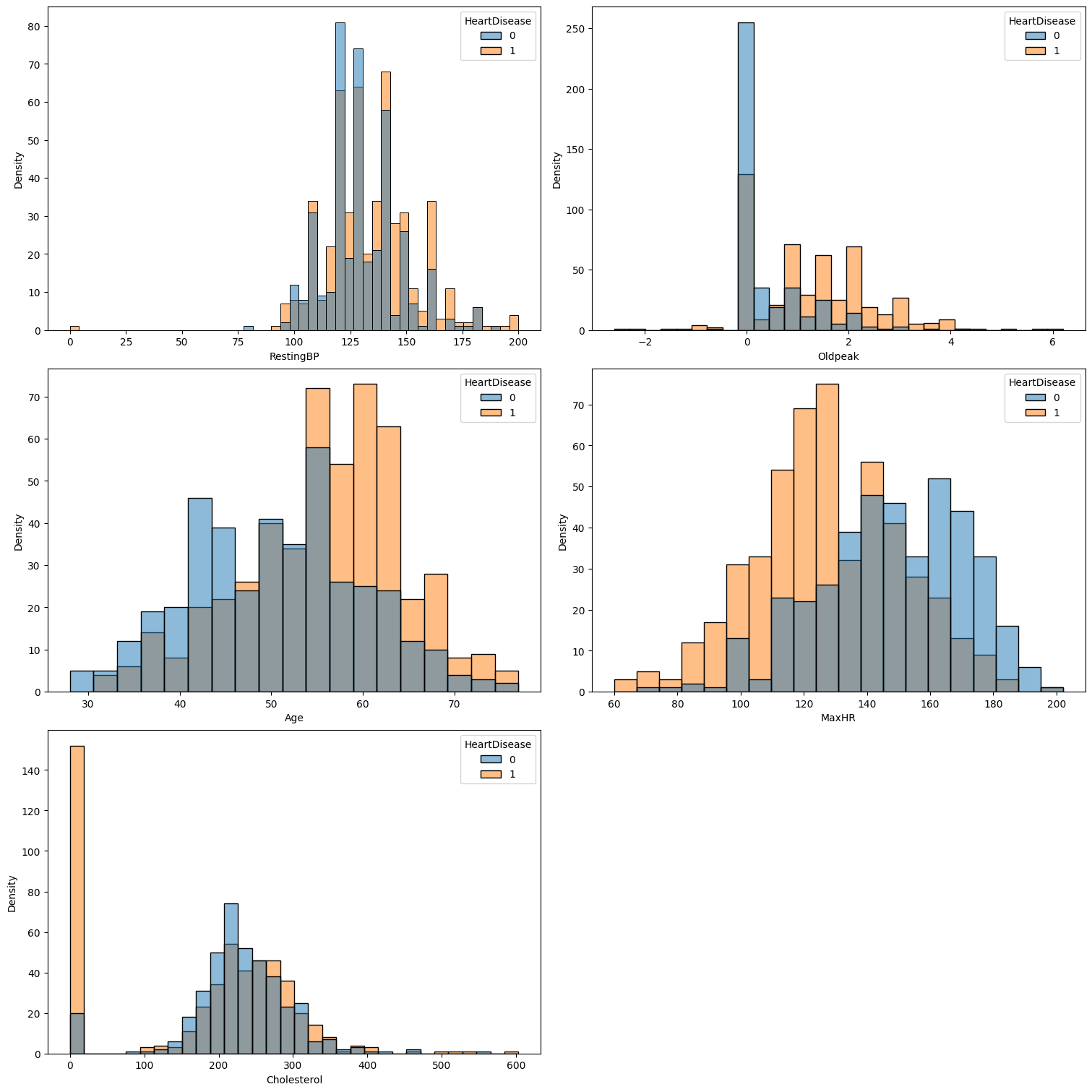
It’s clear that:
Ageshows a strong correlation with heart disease, with older individuals being more likely to develop the condition.Resting Blood Pressure (RestingBP)is inversely related to heart disease risk with lower levels being associated with a reduced likelihood of heart disease.Cholesterol levelspresent a complex relationship with heart disease: both very low and very high cholesterol values are strongly correlated with an increased risk.Maximum Heart Rate (MaxHR)has a negative correlation with heart disease, meaning higher values are associated with a lower risk.- Lower
Oldpeakvalues are generally associated with a reduced likelihood of heart disease. However, there is some overlap at very low values, which can make interpretation more challenging.
RestingBPmay be omitted if further analysis deems it unimportant.
sns.heatmap(df.corr(), annot=True, cmap='coolwarm', fmt='.2f')
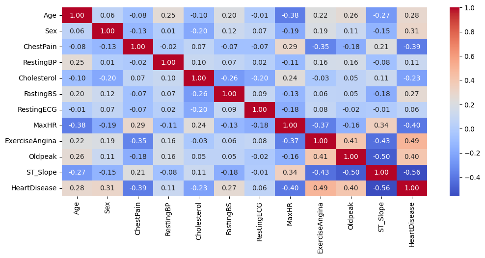
- The correlation matrix reveals a strong correlation between certain features, such as
ST_SlopeandOldpeak. This high correlation can adversely affect the model’s performance. To mitigate this issue, we need to consider strategies to address multicollinearity. Options include dropping one of the correlated features, combining them into a single variable, or selecting a model that is inherently resistant to multicollinearity, such as aDecisionTreeClassifier. - We could also use Principal Component Analysis (PCA) to tackle the issue of multicollinearity, by transforming the original variables into a new set of uncorrelated variables. However, PCA assumes the data is normally distributed, which is not the case here.
df.corr().abs().drop('HeartDisease').nlargest(11, 'HeartDisease')['HeartDisease']
ST_Slope          0.558771
ExerciseAngina    0.494282
Oldpeak           0.403951
MaxHR             0.400421
ChestPain         0.386828
Sex               0.305445
Age               0.282039
FastingBS         0.267291
Cholesterol       0.232741
RestingBP         0.107589
RestingECG        0.057384
Name: HeartDisease, dtype: float64
Our findings are consistent with our previous statements. The data indicates that RestingECG is the feature least correlated with HeartDisease, followed by RestingBP. Additionally, Cholesterol shows a weak correlation with HeartDisease. Notably, the correlation coefficients for these features are all below 0.15. As a result, we will be removing these three features.
Conclusions
- The dataset is balanced and contains no missing values, eliminating the need for imputation, row deletion, or oversampling.
- We conclude that
RestingECG,RestingBP, andCholesterolare not indicative of heart disease and will therefore be excluded from the dataset. - We will OneHotEncoder to encode our categorical features.
- Numerical features are not normally distributed and contain outliers. To address this we will employ RobustScaler.
- We will only consider models that are robust to multicollinearity.
We reverse the encoding of our categorical features to preserve the original values, drop the aforementioned features, and save the preprocessed dataset.
for column in categorical_features:
    if column in df.columns:
        df[column] = encoders[column].inverse_transform(df[column])

df = df.drop(columns=["RestingECG", "RestingBP", "Cholesterol"])
df.to_csv(Path.cwd() / "heart_processed.csv", index=False)
Stay tuned for our next post, where we’ll dive into selecting and training a model using our freshly preprocessed heart disease data. Exciting insights await ❤ !
